
HEOR Dashboard
▶ Try the live dashboard
No install, no sign-up. It runs entirely in your browser on WebAssembly —give it ten seconds to load the R runtime.
You can drop your own master table into it. Open "Use your own data" andload a .csv, .rds, .tsv or .parquet file. Because the page isWebAssembly, R is running inside your browser: the file is read locally andnever crosses the network. Nothing is uploaded to any server, including thisone.
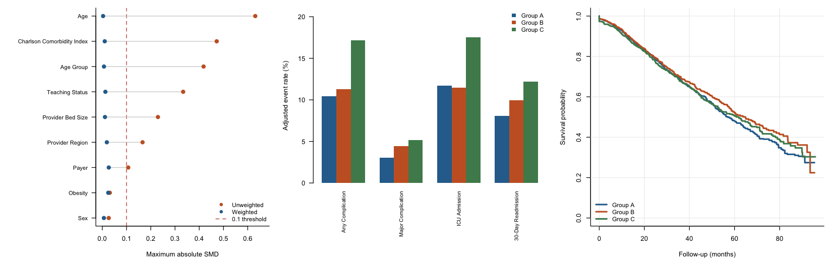
Reusable tooling for health economics and outcomes research on real-worldhealthcare data. Two independent pieces, one idea: an analyst prepares amaster table; the tools do the rest, and every number is computed by testedcode rather than estimated.
The figure is what the package is for. On the left, nine covariates that arebadly imbalanced between treatment groups — age at |SMD| 0.58 — collapse tonear zero after overlap weighting. The middle and right panels are what youare then entitled to compare.
| What it is | |
|---|---|
heorkit/ |
An R package. Give it an episode-level master table and a declaration of what your columns mean; get baseline balance, overlap-weighted outcome comparisons, cost and survival analysis, and an interactive Shiny dashboard. |
heor-mcp/ |
An MCP server exposing the same statistical ideas as deterministic tools an LLM agent can call, so the model orchestrates but never computes. |
Both run end to end on bundled synthetic data. No real, licensed, orproprietary data is in this repository, and none should ever be committed to it.
heorkit
Why it exists
Every HEOR study repeats the same work: build Table 1, check whether thetreatment groups are comparable, adjust for confounding, compare outcomes,caveat the cost figures. The data source changes every time. The analysis doesnot.
So heorkit fixes the analysis and lets the data source vary. There is no SQLin this package on purpose — extraction is specific to your warehouse andlicense, and no shipped query would survive contact with a different schema.What ships is everything downstream of the extract.
Install
# install.packages("remotes")
remotes::install_github("lin-penglin/heorkit", subdir = "heorkit")
Base R plus stats/graphics covers the analysis. nnet improves thepropensity model for 3+ groups, survival enables Kaplan-Meier, andshiny (+ optional DT) powers the dashboard.
Sixty-second tour
No R project, no setup. Two commands from the repo root:
Rscript examples/make_sample_data.R   # writes a 1,000-episode sample table
Rscript examples/run_dashboard.R      # opens the dashboard on it
Or from the R console:
library(heorkit)

data <- heor_synthetic_master_table(n = 5000)   # swap in your own table
spec <- heor_example_spec()                     # or write your own heor_spec()

prepared <- heor_prepare(data, spec)
launch_heor_dashboard(prepared)
The sidebar controls four separate things:
| Control | What it changes |
|---|---|
| Weighting covariates | Which variables enter the propensity model |
| Groups to compare | Which treatment levels are analysed, and which is the reference |
| Outcomes to show | Which outcomes appear in every table and chart |
| Filters | Which episodes are in the cohort |
Dropping a group removes its rows entirely, so the propensity model refits onthe ones you kept — an A-versus-B comparison is weighted toward the A/B overlappopulation, not a three-group one. Selecting a single group gives a descriptiveview with no comparison.
Empty means "all" in each case. The two selections are deliberately independent:narrowing the outcome list never touches the propensity model, so two views ofthe same cohort are always adjusted identically. And when you drop a covariatefrom the model, the balance panel still scores every covariate — includingthe one you removed, which is precisely the one you need to see.
Both are available programmatically too:
heor_select_outcomes(spec, outcomes_binary = c("flag_any_complication",
                                               "flag_readmission_30d"))
heor_overlap_weights(prepared, covariates = c("age", "cci"))
If the sidebar looks out of date after upgrading, restart your R session.R will not reload a package that is already attached, so
library(heorkit)from earlier in the session keeps serving the old UI. The version in thedashboard footer tells you which build is actually running.
examples/ also holds app.R, a ready-to-publishentry point for Shiny Server, Posit Connect, or shinyapps.io. Seedocs/deploying.md for how to share the dashboard with otherpeople — and which routes are safe once real data is involved.
Your own table plugs in by describing it once:
spec <- heor_spec(
  treatment            = "treatment_group",
  baseline_continuous  = c(age = "Age", cci = "Charlson Index"),
  baseline_categorical = c(sex = "Sex", payer = "Payer"),
  outcomes_binary      = c(readmit_30d = "30-Day Readmission"),
  outcomes_cost        = c(total_cost = "Total Cost"),
  time_to_event        = c(time = "followup_months", event = "death")
)
See docs/master_table_contract.md for the fullcontract.
Or skip writing the spec by hand and let the package propose one:
master <- heor_read_master_table("my_extract.parquet")   # csv / rds / tsv / parquet
spec    <- heor_infer_spec(master)                       # a proposal, not a verdict
attr(spec, "inferred")                                   # what it decided, and why

heor_validate(master, spec)
launch_heor_dashboard(heor_prepare(master, spec))
heor_infer_spec() reads column types and names: 0/1 columns become binaryoutcomes, names mentioning cost or charge become economic outcomes, namesmentioning stay, days or visits become utilisation, and everything else numericbecomes a baseline covariate. Check it. Whether a numeric column is acovariate or an outcome is a study-design question, and age andlength_of_stay look identical to a type check — so the function returns aninferred attribute recording every decision it made, and the dashboard'sContract tab shows the same thing.
What it actually does
Confounding by indication is the central problem in this kind of data: thepatients who get the newer treatment are usually younger and healthier, so theraw comparison flatters it. The bundled synthetic data has that confoundingbuilt in deliberately, and the package's job is to remove it.
res <- heor_compare(prepared)
res
#> <heor_comparison> Synthetic Treatment Comparison Study
#>   treatment: treatment_group - Group A vs Group B vs Group C
#>   rows used: 5,000 (0 dropped)
#>   ESS after weighting: Group A = 2,332, Group B = 948, Group C = 850
#>   balance: all 9 covariates within |SMD| <= 0.10 after weighting
Before weighting, the groups are not comparable — and the outcome gap lookslarge:
| Group A | Group B | Group C | |
|---|---|---|---|
| N | 3,135 | 960 | 905 |
| Any Complication | 261 (8.33%) | 110 (11.46%) | 166 (18.34%) |
| 30-Day Readmission | 206 (6.57%) | 74 (7.71%) | 108 (11.93%) |
After overlap weighting, age balances from |SMD| 0.58 to 0.013 and Charlson from0.50 to 0.003 — and roughly a third of the apparent advantage turns out to havebeen case mix:
| Group A | Group B | Group C | |
|---|---|---|---|
| N (effective) | 3,135 (ESS 2,332) | 960 (ESS 948) | 905 (ESS 850) |
| Any Complication | 168 (10.06%) | 199 (11.94%) | 269 (16.15%) |
| 30-Day Readmission | 127 (7.65%) | 133 (8.00%) | 185 (11.10%) |
That shrinkage is the point of the package.
Effect sizes, not just rates
Rates answer "what happened". heor_effect_table() answers "how big is thedifference, and how sure are we" — with HC0 robust confidence intervals, becausea model-based interval under weighting treats the weights as counts and comesout too narrow.
w <- heor_overlap_weights(prepared)
heor_format_effects(heor_effect_table(prepared, weights = w))
#>                   Outcome         Measure         Comparison    Estimate (95% CI)      p
#>          Any Complication      odds ratio Group C vs Group A  1.72 (1.37 to 2.16) <0.001
#>                Total Cost mean difference Group C vs Group A -605 (-1,457 to 247)  0.164
#>   Crossover to Comparator      odds ratio Group C vs Group A        not estimable      -
Binary outcomes report an odds ratio or a risk difference, continuous outcomes amean difference, cost outcomes a difference in currency or a ratio. Passingcovariates = TRUE adds outcome-model adjustment on top of the weighting, whichis doubly robust: consistent if either model is right.
That last row matters. Group C has zero crossovers by construction, so thelogistic model is perfectly separated and the parameter is not identified.An unguarded table would print 0.00 (0.00 to 0.00), p < 0.001 — a precise,highly significant finding about a quantity that cannot be estimated.heorkit detects the degenerate cell and says so instead.
Two more analyses round out the set:
heor_cost_by_outcome(prepared)   # incremental cost attributable to each event
heor_km_risk_table(prepared)     # numbers at risk under the KM curve
heor_bootstrap_effects(prepared) # percentile CIs, propensity refit per replicate
heor_adjust_p(effects)           # Benjamini-Hochberg across the tests shown
The dashboard shows over a hundred tests across its tabs. With 49 on the EffectEstimates tab alone and every null true, the chance of at least one p below 0.05is about 92% — so Benjamini-Hochberg is applied by default, to every table,with the method in the sidebar. Each outcome tab is one family; the EffectEstimates tab lets you pick its own. Column headers name what they hold, q (BH)rather than p. Which tests form a family is a study-design decision, and thepackage says so rather than deciding for you.
heor_cost_by_outcome() fits every outcome together, so each figure is theextra cost associated with that event holding the others fixed — a differentquestion from whether cost differs between groups.
Design decisions worth knowing
- Overlap (ATO) weights, not IPTW. Overlap weights are bounded byconstruction, so no single patient with an extreme propensity score candominate the estimate, and for a binary treatment they achieve exact meanbalance on every covariate in the model. The multi-group generalisationfollows Li & Li (2019).
- Effective sample size is always reported. Weighting down-weightsnon-overlapping patients, so ESS can be far below the row count. A weightedtable that hides this is misleading, so the N row shows both.
- SMDs for balance, p-values for outcomes. SMDs do not depend on samplesize; in a large real-world cohort a balance p-value would flag trivialimbalances as "significant".
- Weighted analyses use robust (sandwich) variances. Two traps here, notone. A t-test or chi-square treats the weights as frequencies and inventssample size; a weighted
lm/glmtreats them as precisions, which is justas wrong and produced standard errors about 15–20% too small on the demo data— an order of magnitude on one p-value. Every weighted comparison uses an HC0sandwich Wald test, and survival switches to a weighted Cox model with arobust variance. Column headers name the test that actually ran.docs/weighted-inference.md shows the numbersagainst a bootstrap, and is explicit that propensity-estimation uncertainty isstill treated as fixed — bootstrap for anything going into a manuscript. - Costs are winsorised and reported median-first, because a handful ofcatastrophic episodes otherwise drives the mean.
- Nothing is imputed. Missing categorical covariates become a visible
"(Missing)"level rather than disappearing into a complete-case filter,because differential missingness between arms is itself a finding.
Tests
Rscript -e 'testthat::test_dir("heorkit/tests/testthat", package = "heorkit")'
349 assertions. They check the weighted estimators against hand computations,the robust variance against the sandwich package, the closed-form overlapweight for binary treatment, the balance claim above, that effect estimatesrecover known odds ratios and incremental costs from simulated data, and thecontract validator's failure modes.
heor-mcp
An MCP server that lets an LLM agent run cohort construction, outcomecomputation, and overlap-weighted comparison as deterministic tools — with aguardrail that flags ambiguous codes instead of guessing. Seeheor-mcp/README.md.
Data policy
This repository contains no real patient data and no licensed databasecontent. The synthetic generators are deterministic and produce data thatresembles no real database's schema.
If you use heorkit against licensed data (Premier PINC AI, FinThrive,Optum, Merative, an internal EHR warehouse, or anything similar), your mastertable, your extraction SQL, and your vendor documentation stay on your side ofthe license. .gitignore blocks *.rds, *.parquet, *.xlsx, and *.zip forexactly this reason — but the responsibility is yours, not the file's.
Repository layout
heorkit/                        the R package (analysis + dashboard)
heor-mcp/                       the MCP server
examples/
  make_sample_data.R            writes a 1,000-episode sample table
  run_dashboard.R               loads it, validates it, opens the dashboard
  app.R                         deployable entry point for hosted Shiny
tools/
  build_demo.R                  compiles the WebAssembly demo
  preflight.sh                  pre-publication check
  check_no_data.sh              the licensed-data guard CI runs
  compare_variance.R            reproduces the variance comparison in the docs
  make_readme_figure.R          regenerates the figure above
docs/
  master_table_contract.md      what your table must contain
  weighted-inference.md         p-values, robust variances, multiplicity
  deploying.md                  getting the dashboard to other people
  img/                          generated figures
NEWS.md                         what changed between versions
PUBLISHING.md                   maintaining and releasing this repo
Function reference
Everything exported, grouped by what it is for. Each has a help page:?heor_effect_table.
| Contract | |
heor_spec() |
Declare what your columns mean |
heor_validate() |
Check a table against a spec before trusting it |
heor_prepare() |
Clean it into analysis-ready form |
heor_contract() |
The expected columns, as a data frame |
| Reading a file | |
heor_read_master_table() |
Read .csv, .tsv, .rds, .parquet |
heor_infer_spec() |
Propose a spec from column types and names |
| Narrowing | |
heor_select_groups() |
Restrict to chosen treatment levels; set the reference |
heor_select_outcomes() |
Restrict which outcomes are reported |
| Weighting and balance | |
heor_overlap_weights() |
Fit the propensity model, compute ATO weights |
heor_smd_table() |
Covariate balance, before against after |
| Descriptive tables | |
heor_baseline_table() |
Table 1 with pairwise SMDs |
heor_binary_table() |
Event counts and rates |
heor_continuous_table() |
Mean (SD) and median (IQR) |
heor_cost_table() |
Winsorised, median-first |
heor_volume_by_year() |
Volume and treatment mix over time |
heor_missingness_table() |
What is missing, and how much |
| Effects and inference | |
heor_effect_table() |
Effect sizes with robust confidence intervals |
heor_format_effects() |
Render them for a report |
heor_adjust_p() |
Benjamini-Hochberg, Holm, Bonferroni, BY |
heor_bootstrap_effects() |
Percentile intervals, propensity refit per replicate |
heor_cost_by_outcome() |
Incremental cost attributable to each event |
heor_compare() |
Every table, unadjusted and weighted, in one call |
| Survival | |
heor_km_data() |
Kaplan-Meier coordinates for plotting |
heor_survival_table() |
Survival at fixed times, with pairwise tests |
heor_km_risk_table() |
Numbers at risk |
| Dashboard | |
launch_heor_dashboard() |
Open it |
heor_dashboard_app() |
The app object, for deployment |
| Data and helpers | |
heor_synthetic_master_table() |
Deterministic synthetic data |
heor_example_spec() |
A complete spec for it |
heor_winsorize() |
Cap a heavy-tailed vector |
heor_weighted_mean(), heor_weighted_sd(), heor_weighted_quantile() |
Weighted summaries |
heor_effective_sample_size() |
Kish's ESS |
NEWS.md records what changed between versions — including twocorrections to how weighted p-values are computed, which change publishednumbers.
Publishing or maintaining this repo? See PUBLISHING.md, and runbash tools/preflight.sh before pushing.
License
MIT — see LICENSE.
All results are exploratory and subject to real-world-data limitations.Overlap-weighted estimates target the overlap population, not the full cohort.


